import numpy as np
import matplotlib.pyplot as plt
import pandas as pd
from sklearn.preprocessing import RobustScaler
plt.style.use("bmh")
import ta
from datetime import timedelta
from keras.models import Sequential
from keras.layers import LSTM, Dense, Dropout
df = pd.read_csv("USDTRY=X.csv")
df['Date'] = pd.to_datetime(df.Date)
# Setting the index
df.set_index('Date', inplace=True)
# Dropping any NaNs
df.dropna(inplace=True)
# Adding all the indicators
df = ta.add_all_ta_features(df, open="Open", high="High", low="Low", close="Close", volume="Volume", fillna=True)
# Dropping everything else besides 'Close' and the Indicators
df.drop(['Open', 'High', 'Low', 'Adj Close', 'Volume'], axis=1, inplace=True)
# Checking the new df with indicators
print(df.shape)
# Only using the last 1000 days of data to get a more accurate representation of the current climate
df = df.tail(1000)
# Scale fitting the close prices separately for inverse_transformations purposes later
close_scaler = RobustScaler()
close_scaler.fit(df[['Close']])
# Normalizing/Scaling the Data
scaler = RobustScaler()
df = pd.DataFrame(scaler.fit_transform(df), columns=df.columns, index=df.index)
# Plotting the Closing Prices
df['Close'].plot(figsize=(16,5))
plt.title("Satis Fiyati")
plt.ylabel("Fiyat(olcekli)")
# plt.show()
def split_sequence(seq, n_steps_in, n_steps_out):
"""
Splits the multivariate time sequence
"""
# Creating a list for both variables
X, y = [], []
for i in range(len(seq)):
# Finding the end of the current sequence
end = i + n_steps_in
out_end = end + n_steps_out
# Breaking out of the loop if we have exceeded the dataset's length
if out_end > len(seq):
break
# Splitting the sequences into: x = past prices and indicators, y = prices ahead
seq_x, seq_y = seq[i:end, :], seq[end:out_end, 0]
X.append(seq_x)
y.append(seq_y)
return np.array(X), np.array(y)
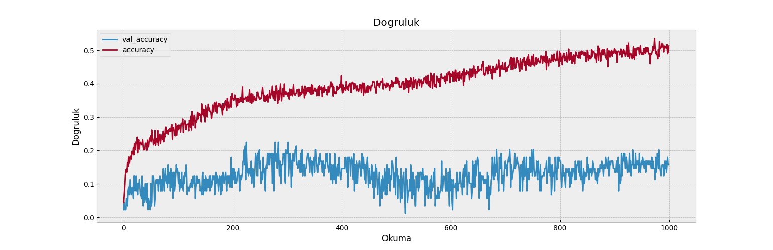
def visualize_training_results(results):
"""
Plots the loss and accuracy for the training and testing data
"""
history = results.history
plt.figure(figsize=(16,5))
plt.plot(history['val_loss'])
plt.plot(history['loss'])
plt.legend(['val_loss', 'loss'])
plt.title('Loss')
plt.xlabel('Epochs')
plt.ylabel('Loss')
plt.show()
plt.figure(figsize=(16,5))
plt.plot(history['val_accuracy'])
plt.plot(history['accuracy'])
plt.legend(['val_accuracy', 'accuracy'])
plt.title('Dogruluk')
plt.xlabel('Okuma')
plt.ylabel('Dogruluk')
plt.show()
def layer_maker(n_layers, n_nodes, activation, drop=None, d_rate=.5):
"""
Creates a specified number of hidden layers for an RNN
Optional: Adds regularization option - the dropout layer to prevent potential overfitting (if necessary)
"""
# Creating the specified number of hidden layers with the specified number of nodes
for x in range(1,n_layers+1):
model.add(LSTM(n_nodes, activation=activation, return_sequences=True))
# Adds a Dropout layer after every Nth hidden layer (the 'drop' variable)
try:
if x % drop == 0:
model.add(Dropout(d_rate))
except:
pass
def validater(n_per_in, n_per_out):
"""
Runs a 'For' loop to iterate through the length of the DF and create predicted values for every stated interval
Returns a DF containing the predicted values for the model with the corresponding index values based on a business day frequency
"""
# Creating an empty DF to store the predictions
predictions = pd.DataFrame(index=df.index, columns=[df.columns[0]])
for i in range(1, len(df)-n_per_in, n_per_out):
# Creating rolling intervals to predict off of
x = df[-i - n_per_in:-i]
# Predicting using rolling intervals
yhat = model.predict(np.array(x).reshape(1, n_per_in, n_features))
# Transforming values back to their normal prices
yhat = close_scaler.inverse_transform(yhat)[0]
# DF to store the values and append later, frequency uses business days
pred_df = pd.DataFrame(yhat,
index=pd.date_range(start=x.index[-1]+timedelta(days=1),
periods=len(yhat),
freq="B"),
columns=[x.columns[0]])
# Updating the predictions DF
predictions.update(pred_df)
return predictions
def val_rmse(df1, df2):
"""
Calculates the root mean square error between the two Dataframes
"""
df = df1.copy()
# Adding a new column with the closing prices from the second DF
df['close2'] = df2.Close
# Dropping the NaN values
df.dropna(inplace=True)
# Adding another column containing the difference between the two DFs' closing prices
df['diff'] = df.Close - df.close2
# Squaring the difference and getting the mean
rms = (df[['diff']]**2).mean()
# Returning the sqaure root of the root mean square
return float(np.sqrt(rms))
# How many periods looking back to learn
n_per_in = 30
# How many periods to predict
n_per_out = 10
# Features
n_features = df.shape[1]
# Splitting the data into appropriate sequences
X, y = split_sequence(df.to_numpy(), n_per_in, n_per_out)
# Instatiating the model
model = Sequential()
# Activation
activ = "tanh"
# Input layer
model.add(LSTM(90,
activation=activ,
return_sequences=True,
input_shape=(n_per_in, n_features)))
# Hidden layers
layer_maker(n_layers=2,
n_nodes=30,
activation=activ,
drop=1,
d_rate=.1)
# Final Hidden layer
model.add(LSTM(90, activation=activ))
# Output layer
model.add(Dense(n_per_out))
# Model summary
model.summary()
# Compiling the data with selected specifications
model.compile(optimizer='adam', loss='mse', metrics=['accuracy'])
res = model.fit(X, y, epochs=2, batch_size=32, validation_split=0.1)
visualize_training_results(res)
# Transforming the actual values to their original price
actual = pd.DataFrame(close_scaler.inverse_transform(df[["Close"]]),
index=df.index,
columns=[df.columns[0]])
# Getting a DF of the predicted values to validate against
predictions = validater(n_per_in, n_per_out)
# Printing the RMSE
print("RMSE:", val_rmse(actual, predictions))
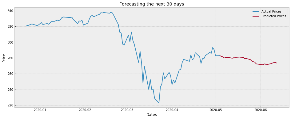
# Plotting
plt.figure(figsize=(16,6))
# Plotting those predictions
plt.plot(predictions, label='Tahmin edilen')
# Plotting the actual values
plt.plot(actual, label='Gerçek')
plt.title(f"Tahmin ve Gercek Fiyat")
plt.ylabel("Fiyat")
plt.legend()
plt.show()
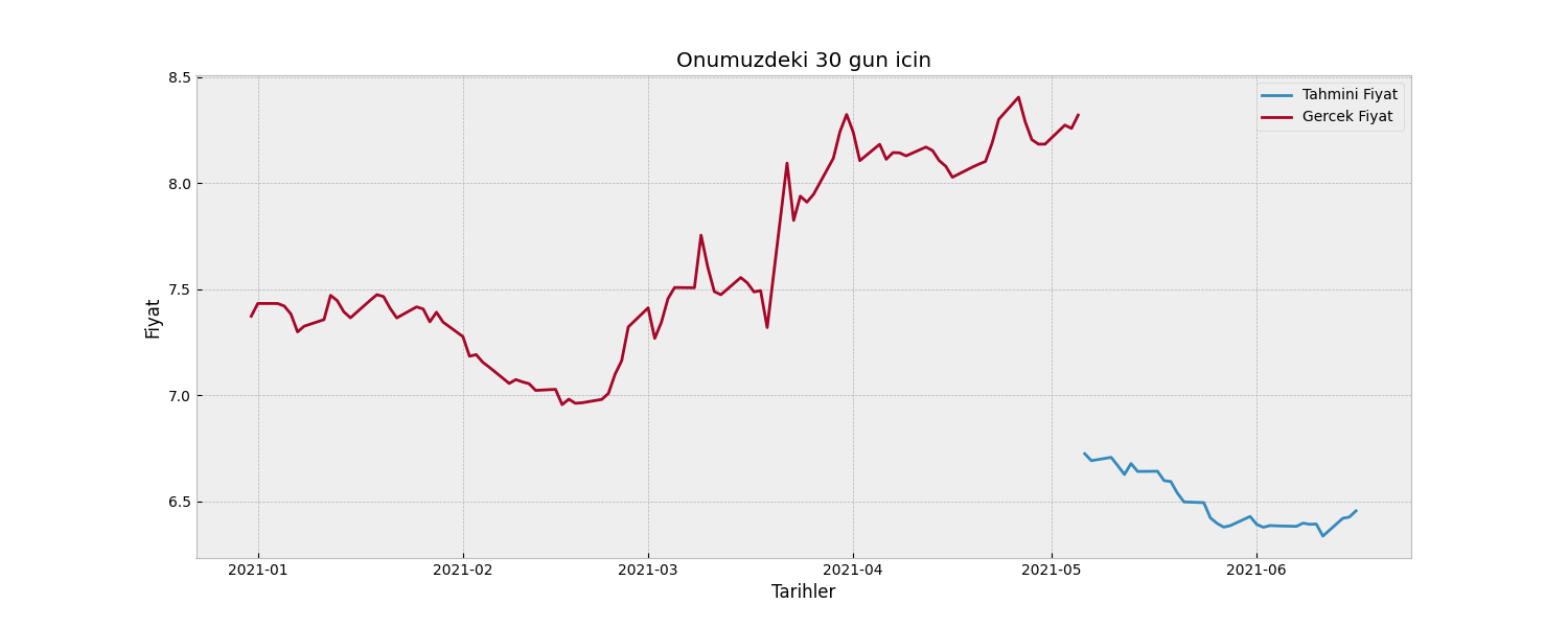
# Predicting off of the most recent days from the original DF
yhat = model.predict(np.array(df.tail(n_per_in)).reshape(1, n_per_in, n_features))
# Transforming the predicted values back to their original format
yhat = close_scaler.inverse_transform(yhat)[0]
# Creating a DF of the predicted prices
preds = pd.DataFrame(yhat,
index=pd.date_range(start=df.index[-1]+timedelta(days=1),
periods=len(yhat),
freq="B"),
columns=[df.columns[0]])
# Number of periods back to plot the actual values
pers = n_per_in
# Transforming the actual values to their original price
actual = pd.DataFrame(close_scaler.inverse_transform(df[["Close"]].tail(pers)),
index=df.Close.tail(pers).index,
columns=[df.columns[0]]).append(preds.head(1))
# Printing the predicted prices
print(preds)
# Plotting
plt.figure(figsize=(15,6))
plt.plot(preds, label="Tahmini Fiyat")
plt.plot(actual, label="Gercek Fiyat")
plt.ylabel("Fiyat")
plt.xlabel("Tarihler")
plt.title(f"Onumuzdeki {len(yhat)} gun icin")
plt.legend()
plt.show()Merhabalar,
Elimde bu şekilde bir kod var. Kodun mantığını kabaca anladım. Fakat gelecek günkü tahminlerde grafikte bozulma oluyor(Screenshot by Lightshot). Dolar ile alakası yok. BTC EUR filan hepsinde oluyor aynı şey. Kur geçmişini yahoo finance den alıyorum.
Kodun orijinal hali burada (Price-Forecaster/Stock-RNN-Deep-Learning-TechIndicators.ipynb at master · marcosan93/Price-Forecaster · GitHub)
Bu sayfadaki " Validating the Model" kısmından hata verdiği için plt.xlim('2018-05', '2020-05') burayı çıkarttım ve çıkarttıktan sonra hata vermemeye başladı. Bu hatayı verdiği yer “tahmin ve gerçek fiyat” grafiği, “gelecek günkü tahmin” grafiği ile alakası yok gibi ama sizce grafikteki problem burayı çıkarttığım için mi oldu ? Sizce grafikte bozulma neden oluyor ve nasıl düzeltebilirim ?